

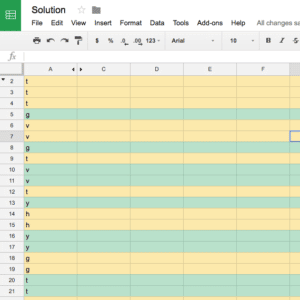
Here are step-by-step instructions on how you can use conditional formatting to alternate the row color when a value changes in Google Sheets. This is a great trick to know in order to increase visibility on a busy spreadsheet that contains duplicates. For this example, our data is in Column A.
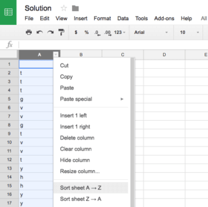
If it isn’t already in alphabetic or numeric order, sort your spreadsheet A→Z from the column of data that you will be conditionally formatting.
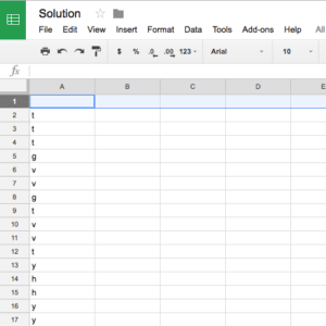
If there isn’t one already, you will need to insert a blank row above your first row of data. The way this formula was written requires that this row stay blank. For cleaner viewing, this row can be hidden. It doesn’t matter if your cells do not begin at A1 and A2, there just needs to be a blank row in front of your first cell of data.
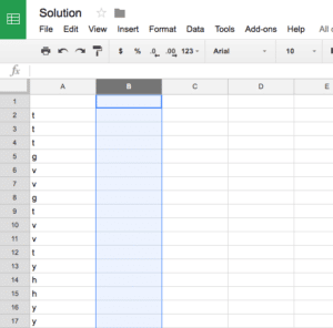
You’ll also need to insert or designate a blank column somewhere on the spreadsheet to be the ‘helper’ column. This column will hold the formula which triggers the conditional formatting in the column where your data is (in this example – Column B). For cleaner viewing, this column can be hidden.
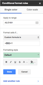
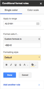
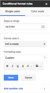
Start by applying the following conditional formatting rules to the column your data is in. Make sure each rule has a different designated color. Also, your range will include all of the cells in the column where your data is except for the first blank cell in the row you inserted. The conditional formatting, as you’ll see, references your helper column not your data column. There are 3 rules you will need:
- Custom formula =$B2=1
- Custom formula =B2=0
- Cell is empty
*In order to highlight the entire row/spreadsheet, as opposed to just the cells in our data column, we extended our range from A2:Z1001. To keep the coloring contained in the column, we would make our range A2:A1001.

Now, in the cell of your helper column that corresponds with the first cell of data in your data column, B2 in this example, insert the following formula and copy it all the way down. Make sure to change cell letters/numbers accordingly to the letter of your data/helper column if it is not the same as ours:
=MOD(IF(ROW()=2,0,IF(A2=A1,B1, B1+1)), 2)
Happy formatting!